LinuxClustering.net

Establish Basic Rate of Change

First, use these commands to determine the basic daily rate of change for the files or partitions that you want to mirror; for example, to measure the amount of data written in a day for /dev/sda3, run this command at the beginning of the day:

MB_START=`awk ‘/sda3 / { print $10 / 2 / 1024 }’ /proc/diskstats`

Wait for 24 hours, then run this command:

MB_END=`awk ‘/sda3 / { print $10 / 2 / 1024 }’ /proc/diskstats`

The daily rate of change, in megabytes, is then MB_END – MB_START.

The amounts of data that you can push through various network connections are as follows:

• For T1 (1.5Mbps): 14,000 MB/day (14 GB)
• For T3 (45Mbps): 410,000 MB/day (410 GB)
• For Gigabit (1Gbps): 5,000,000 MB/day (5 TB)

Establish Detailed Rate of Change

Next, you’ll need to measure detailed rate of change. The best way to collect this data is to log disk write activity for some period (e.g., one day) to determine the peak disk write periods. To do so, create a cron job that will log the timestamp of the system followed by a dump of /proc/diskstats. For example, to collect disk stats every 2 minutes, add this link to /etc/crontab:

*/2 * * * * root ( date ; cat /proc/diskstats ) >> /path_to/filename.txt

Wait for the determined period (e.g., one day, one week), then disable the cron job and save the resulting /proc/diskstats output file in a safe location.

Analyze and Graph Detailed Rate of Change Data

Next you should analyze the detailed rate of change data. You can use the roc-calc-diskstats utility for this task. This utility takes the /proc/diskstats output file and calculates the rate of change of the disks in the dataset. To run the utility, use this command:

# ./roc-calc-diskstats <interval> <start_time> <diskstats-data-file> [dev-list]

For example, the following dumps a summary (with per-disk peak I/O information) to the output file results.txt:

# ./roc-calc-diskstats 2m “Jul 22 16:04:01” /root/diskstats.txt sdb1,sdb2,sdc1 > results.txt

Here are sample results from the results.txt file:

Sample start time: Tue Jul 12 23:44:01 2011

Sample end time: Wed Jul 13 23:58:01 2011

Sample interval: 120s #Samples: 727 Sample length: 87240s

(Raw times from file: Tue Jul 12 23:44:01 EST 2011, Wed Jul 13 23:58:01 EST 2011)

Rate of change for devices dm-31, dm-32, dm-33, dm-4, dm-5, total

dm-31 peak:0.0 B/s (0.0 b/s) (@ Tue Jul 12 23:44:01 2011) average:0.0 B/s (0.0 b/s)

dm-32 peak:398.7 KB/s (3.1 Mb/s) (@ Wed Jul 13 19:28:01 2011) average:19.5 KB/s (156.2 Kb/s)

dm-33 peak:814.9 KB/s (6.4 Mb/s) (@ Wed Jul 13 23:58:01 2011) average:11.6 KB/s (92.9 Kb/s)

dm-4 peak:185.6 KB/s (1.4 Mb/s) (@ Wed Jul 13 15:18:01 2011) average:25.7 KB/s (205.3 Kb/s)

dm-5 peak:2.7 MB/s (21.8 Mb/s) (@ Wed Jul 13 10:18:01 2011) average:293.0 KB/s (2.3 Mb/s)

total peak:2.8 MB/s (22.5 Mb/s) (@ Wed Jul 13 10:18:01 2011) average:349.8 KB/s (2.7 Mb/s)

To help you understand your specific bandwidth needs over time, you can graph the detailed rate of change data. The following dumps graph data to results.csv (as well as dumping the summary to results.txt):

# export OUTPUT_CSV=1

# ./roc-calc-diskstats 2m “Jul 22 16:04:01” /root/diskstats.txt sdb1,sdb2,sdc1 2> results.csv > results.txt

SIOS has created a template spreadsheet, diskstats-template.xlsx, which contains sample data that you can overwrite with your data from roc-calc-diskstats. The following series of images show the process of using the spreadsheet.

1. Open results.csv, and select all rows, including the total column.

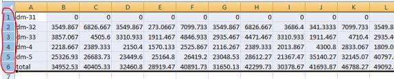
2. Open diskstats-template.xlsx, select the diskstats.csv worksheet.

3. In cell 1-A, right-click and select Insert Copied Cells.
4. Adjust the bandwidth value in the cell towards the bottom left of the worksheet (as marked in the following figure) to reflect the amount of bandwidth (in megabits per second) that you have allocated for replication. The cells to the right are automatically converted to bytes per second to match the collected raw data.

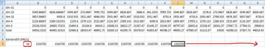
5. Take note of the following row and column numbers:

• Total (row 6 in the following figure)
• Bandwidth (row 9 in the following figure)
• Last datapoint (column R in the following figure)

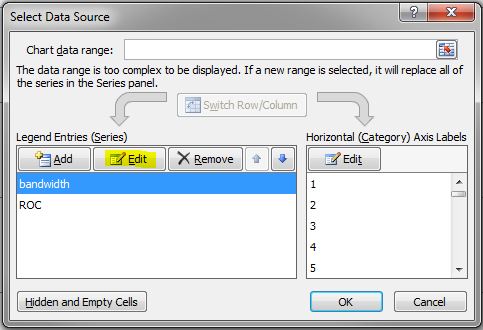
6. Select the bandwidth vs ROC worksheet.

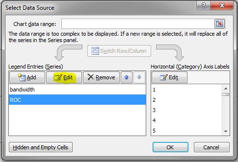
7. Right-click the graph and choose Select Data.
8. In the Select Data Source dialog box, choose bandwidth in the Legend Entries (Series) list, and then click Edit.

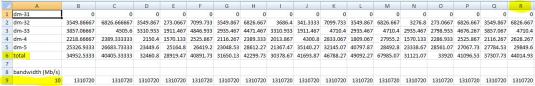
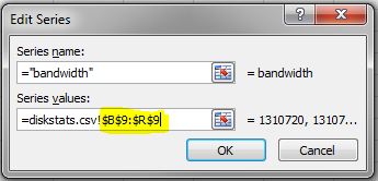
9. In the Edit Series dialog box, use the following syntax in the Series values field: =diskstats.csv!$B$<row>:$<final_column>$<row> The following figure shows the series values for the spread B9 to R9.

10. Click OK to close the Edit Series box.
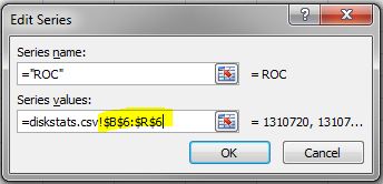
11. In the Select Data Source box, choose ROC in the Legend Entries (Series) list, and then click Edit.

12. In the Edit Series dialog box, use the following syntax in the Series values field: =diskstats.csv!$B$<row>:$<final_column>$<row> The following figure shows the series values for the spread B6 to R6.

13. Click OK to close the Edit Series box, then click OK to close the Select Data Source box.

The Bandwidth vs ROC graph updates. Analyze your results to determine whether you have sufficient bandwidth to support data replication.

Next Steps

If your Rate of Change exceeds your available bandwidth, you will need to consider some of the following points to ensure your replication solution performs optimally:

• Enable compression in your replication solution or in the network hardware. (DataKeeper for Linux, which is part of the SteelEye Protection Suite for Linux, supports this type of compression.)
• Create a local, non-replicated storage repository for temporary data and swap files that don’t need to be replicated.
• Reduce the amount of data being replicated.
• Increase your network capacity.